pymc3 快速入门
原文链接: https://docs.pymc.io/notebooks/api_quickstart.html
翻译者: 小夏 ([email protected])
声明: 本人不负责回答任何与该文档有关的问题, 如需向我提问, 请访问 https://www.notion.so/dddd1007/fa9af18679064c56a4976ca350d0b3cd 并按内容操作.
%matplotlib inline
import numpy as np
import theano.tensor as tt
import pymc3 as pm

import seaborn as sns
import matplotlib.pyplot as plt

sns.set_context('notebook')
plt.style.use('seaborn-darkgrid')
print('Running on PyMC3 v{}'.format(pm.__version__))
Running on PyMC3 v3.8
1. 模型构建
PyMC3 中, 我们围绕着 Model 类这个概念来构建对象. 在这个对象当中, 需要包含全部的随机变量 (Random Variable, RVs), 并在对象内根据梯度函数计算相关参数. 一般情况下, 你可以用一段 with 开头的语句, 通过上下文来构建一个 PyMC3 模型实例. 如下所示:
with pm.Model() as model:
    # 定义模型当中的变量
    pass
在这里我们补充一下
with as结构与上下文的概念.
在 PyMC3 中, 所有的模型均是一个 Model 对象, 而初始化这个对象时, 并非使用
Model()来建立实例, 而是使用with语句. 其原因是 Model 类被构建为一个上下文管理器 (contextor), 在使用 with 调用时, 会执行其中的__enter__与__exit__魔法方法所定义的命令, 从而自动完成一系列任务的执行.
with [as var]当中的as var部分并不是必要的, 但如果有as var部分, 则会将执行魔法方法的结果赋值给 var 对象.
我们会在后面具体探讨随机变量, 不过在这里先通过一些高斯变量构建一个简单的模型, 来理解一下 Model 类.
with pm.Model() as model:
    mu = pm.Normal("mu", mu=0, sigma=1)
    obs = pm.Normal("obs", mu=mu, sigma=1, observed=np.random.randn(100))
接下来我们查看一下模型的基本信息:
- 包含的随机变量
- 包含的自由随机变量
- 模型中的已观测变量
- 模型中参数的对数概率
print(model.basic_RVs)

print(model.free_RVs)

print(model.observed_RVs)

print(model.logp({"mu":0}))

print(model.logp({"mu":2}))
[mu, obs]
[mu]
[obs]
-140.46697659984773
-350.2760689188665
我们解释一下 logp (即 Log probability, 对数概率). 对数概率是在计算机科学领域和概率论中常用的表征概率的方法, 可以将标准的
[0,1]概率映射到更大的范围上, 从而提高计算精度与效率.
需要注意的是, 在 PyMC3 中, 可以直接使用 logp 方法将对数概率以属性的方式呈现, 但这个值并非静态的. 因此如果你需要在后续的计算中调用 logp 的取值的话, 你需要先将变量静态化, 从而提高运算效率. 具体的例子如下:
%timeit model.logp({mu: 0.1})
logp = model.logp
%timeit logp({mu: 0.1})
64.3 ms ± 2.55 ms per loop (mean ± std. dev. of 7 runs, 10 loops each)
20.7 µs ± 279 ns per loop (mean ± std. dev. of 7 runs, 100000 loops each)
2. 概率分布
在所有的概率程序中, 都包含了被观测的或未被观测到的随机变量. 被观测到的随机变量可以通过其似然分布来定义, 而未被观测到的变量则需要通过相应的先验分布来描述. 在 PyMC3 中, 调用的主模块空间当中便包含了常用的概率分布. 我们先来看下正态分布:
help(pm.Normal)
Help on class Normal in module pymc3.distributions.continuous:

class Normal(pymc3.distributions.distribution.Continuous)
 |  Normal(name, *args, **kwargs)
 |
 |  Univariate normal log-likelihood.
 |
 |  The pdf of this distribution is
 |
 |  .. math::
 |
 |     f(x \mid \mu, \tau) =
 |         \sqrt{\frac{\tau}{2\pi}}
 |         \exp\left\{ -\frac{\tau}{2} (x-\mu)^2 \right\}
 |
 |  Normal distribution can be parameterized either in terms of precision
 |  or standard deviation. The link between the two parametrizations is
 |  given by
 |
 |  .. math::
 |
 |     \tau = \dfrac{1}{\sigma^2}
 |
 |  .. plot::
 |
 |      import matplotlib.pyplot as plt
 |      import numpy as np
 |      import scipy.stats as st
 |      plt.style.use('seaborn-darkgrid')
 |      x = np.linspace(-5, 5, 1000)
 |      mus = [0., 0., 0., -2.]
 |      sigmas = [0.4, 1., 2., 0.4]
 |      for mu, sigma in zip(mus, sigmas):
 |          pdf = st.norm.pdf(x, mu, sigma)
 |          plt.plot(x, pdf, label=r'$\mu$ = {}, $\sigma$ = {}'.format(mu, sigma))
 |      plt.xlabel('x', fontsize=12)
 |      plt.ylabel('f(x)', fontsize=12)
 |      plt.legend(loc=1)
 |      plt.show()
 |
 |  ========  ==========================================
 |  Support   :math:`x \in \mathbb{R}`
 |  Mean      :math:`\mu`
 |  Variance  :math:`\dfrac{1}{\tau}` or :math:`\sigma^2`
 |  ========  ==========================================
 |
 |  Parameters
 |  ----------
 |  mu: float
 |      Mean.
 |  sigma: float
 |      Standard deviation (sigma > 0) (only required if tau is not specified).
 |  tau: float
 |      Precision (tau > 0) (only required if sigma is not specified).
 |
 |  Examples
 |  --------
 |  .. code-block:: python
 |
 |      with pm.Model():
 |          x = pm.Normal('x', mu=0, sigma=10)
 |
 |      with pm.Model():
 |          x = pm.Normal('x', mu=0, tau=1/23)
 |
 |  Method resolution order:
 |      Normal
 |      pymc3.distributions.distribution.Continuous
 |      pymc3.distributions.distribution.Distribution
 |      builtins.object
 |
 |  Methods defined here:
 |
 |  __init__(self, mu=0, sigma=None, tau=None, sd=None, **kwargs)
 |      Initialize self.  See help(type(self)) for accurate signature.
 |
 |  logcdf(self, value)
 |      Compute the log of the cumulative distribution function for Normal distribution
 |      at the specified value.
 |
 |      Parameters
 |      ----------
 |      value: numeric
 |          Value(s) for which log CDF is calculated. If the log CDF for multiple
 |          values are desired the values must be provided in a numpy array or theano tensor.
 |
 |      Returns
 |      -------
 |      TensorVariable
 |
 |  logp(self, value)
 |      Calculate log-probability of Normal distribution at specified value.
 |
 |      Parameters
 |      ----------
 |      value: numeric
 |          Value(s) for which log-probability is calculated. If the log probabilities for multiple
 |          values are desired the values must be provided in a numpy array or theano tensor
 |
 |      Returns
 |      -------
 |      TensorVariable
 |
 |  random(self, point=None, size=None)
 |      Draw random values from Normal distribution.
 |
 |      Parameters
 |      ----------
 |      point: dict, optional
 |          Dict of variable values on which random values are to be
 |          conditioned (uses default point if not specified).
 |      size: int, optional
 |          Desired size of random sample (returns one sample if not
 |          specified).
 |
 |      Returns
 |      -------
 |      array
 |
 |  ----------------------------------------------------------------------
 |  Data and other attributes defined here:
 |
 |  data = array([ 0.55846269, -0.94256117,  0.25300367, -0...22287042,  1...
 |
 |  ----------------------------------------------------------------------
 |  Methods inherited from pymc3.distributions.distribution.Distribution:
 |
 |  __getnewargs__(self)
 |
 |  __latex__ = _repr_latex_(self, name=None, dist=None)
 |      Magic method name for IPython to use for LaTeX formatting.
 |
 |  default(self)
 |
 |  get_test_val(self, val, defaults)
 |
 |  getattr_value(self, val)
 |
 |  logp_nojac(self, *args, **kwargs)
 |      Return the logp, but do not include a jacobian term for transforms.
 |
 |      If we use different parametrizations for the same distribution, we
 |      need to add the determinant of the jacobian of the transformation
 |      to make sure the densities still describe the same distribution.
 |      However, MAP estimates are not invariant with respect to the
 |      parametrization, we need to exclude the jacobian terms in this case.
 |
 |      This function should be overwritten in base classes for transformed
 |      distributions.
 |
 |  logp_sum(self, *args, **kwargs)
 |      Return the sum of the logp values for the given observations.
 |
 |      Subclasses can use this to improve the speed of logp evaluations
 |      if only the sum of the logp values is needed.
 |
 |  ----------------------------------------------------------------------
 |  Class methods inherited from pymc3.distributions.distribution.Distribution:
 |
 |  dist(*args, **kwargs) from builtins.type
 |
 |  ----------------------------------------------------------------------
 |  Static methods inherited from pymc3.distributions.distribution.Distribution:
 |
 |  __new__(cls, name, *args, **kwargs)
 |      Create and return a new object.  See help(type) for accurate signature.
 |
 |  ----------------------------------------------------------------------
 |  Data descriptors inherited from pymc3.distributions.distribution.Distribution:
 |
 |  __dict__
 |      dictionary for instance variables (if defined)
 |
 |  __weakref__
 |      list of weak references to the object (if defined)
在 PyMC3 的模块中, 概率分布包含了:
- 连续型
- 离散型
- 时间序列型
- 混合型
2.1 未被观测到的随机变量
调用未被观测到的随机变量时需要输入变量名称 (字符串形式) 与关键的模型参数. 因此, 一个正态分布可以用如下方式定义:
with pm.Model():
    x = pm.Normal('x', mu=0, sigma=1)
此时我们同样可以计算其对数概率:
x.logp({'x': 0})
array(-0.91893853)
2.2 观测到的随机变量
定义被观测到的随机变量时基本与上面的示例相同, 唯一要注意的是需要将观测到的变量以 observed 参数输入:
with pm.Model():
    obs = pm.Normal('x', mu=0, sigma=1, observed=np.random.randn(100))
observed 可以以列表, numpy数组, theano 或者 pandas 的数据结构输入.
2.3 随机变量的确定性变换
PyMC3 甚至允许你将随机变量像常量一样自由地进行代数运算:
with pm.Model():
    x = pm.Normal('x', mu=0, sigma=1)
    y = pm.Gamma('y', alpha=1, beta=1)

    plus_2 = x + 2
    summed = x + y
    squared = x**2
    sined = pm.math.sin(x)
尽管这种变换近乎无缝衔接 (无需先存为静态数据再进行计算的过程), 然而相应的结果也并未自动保存. 因此, 如果你希望能够追踪这些被变换过的变量的变化, 你需要使用 pm.Deterministic 函数:
with pm.Model():
    x = pm.Normal('x', mu=0, sigma=1)
    plus_2 = pm.Deterministic('x plus 2', x + 2)
注意这里的 plus_2 的表达方式, 我们告诉 PyMC3 只需为我们追踪这一个变量即可.
2.4 有边界随机变量 (bounded RVs) 的自动变换
为了使模型计算更加有效率, PyMC3 会自动将有边界的随机变量变换为无边界变量.
with pm.Model() as model:
    x = pm.Uniform('x', lower=0, upper=1)
当我们查看模型中的随机变量时, 我们预期看到的是上面模型中定义的 x 变量. 然而:
model.free_RVs
[x_interval__]
显示结果中的 x_interval__ 表示 x 已经变换为 [-inf, +inf] 的一个参数传入到模型中. 本例子中的上下界已经经过了一个 LogOdds (对数) 变换. 这个变换使得采样变得更加容易一些. 当然, PyMC3 也会追踪未经变换, 仍包含着边界的参数变化. 查看对象中的 determinstics 属性便可以看到:
model.deterministics
[x]
在显示结果时, PyMC3 往往会隐藏变换参数的过程. 你可以传入 include_transformed=True 到函数中来查看是否是使用变换后的参数来进行取样的.
如果你不喜欢这种自动变换, 你可以把它关掉, 只需传入 transform=None 参数即可:
with pm.Model() as model:
    x = pm.Uniform('x', lower=0, upper=1, transform=None)

print(model.free_RVs)
[x]
或者指定特定的变换形式:
import pymc3.distributions.transforms as tr

with pm.Model() as model:
    # 默认的变换形式
    x1 = pm.Gamma('x1', alpha=1, beta=1)
    # 指定其他的变换形式
    x2 = pm.Gamma('x2', alpha=1, beta=1, transform=tr.log_exp_m1)

print('x1 使用默认的参数变换是:' + x1.transformation.name)
print('x2 所指定的变换是:' + x2.transformation.name)
x1 使用默认的参数变换是:log
x2 所指定的变换是:log_exp_m1
2.5 分布变换与变量的改变
PyMC3 并不直接提供专门将一个分布变换为另一个分布的函数. 恰恰相反, 为了优化性能, PyMC3 会新创建一个特定的分布. 不过用户还是可以通过 transform 传入逆变换参数来进行分布变换. 我们在这里呈现一个经典 LogNormal 范例: $\log (y) \sim \operatorname{Normal}(\mu, \sigma)$
class Exp(tr.ElemwiseTransform):
    name = "exp"

    def backward(self, x):
        return tt.log(x)

    def forward(self, x):
        return tt.exp(x)

    def jacobian_det(self, x):
        return -tt.log(x)

with pm.Model() as model:
    x1 = pm.Normal('x1', 0., 1., transform=Exp()) # 这里传入了 Exp() 作为 transform 参数
    x2 = pm.Lognormal('x2', 0., 1.)

lognorm1 = model.named_vars['x1_exp__'] # named_vars 属性为指定名称的随机变量
lognorm2 = model.named_vars['x2']
x = np.linspace(0., 10., 100)

#
_, ax = plt.subplots(1, 1, figsize=(5, 3))
ax.plot(
    x,
    np.exp(lognorm1.distribution.logp(x).eval()),
    '--',
    alpha=.5,
    label='log(y) ~ Normal(0, 1)')
ax.plot(
    x,
    np.exp(lognorm2.distribution.logp(x).eval()),
    alpha=.5,
    label='y ~ Lognormal(0, 1)')
plt.legend();

我们可以看到上述的两个分布完全一致.
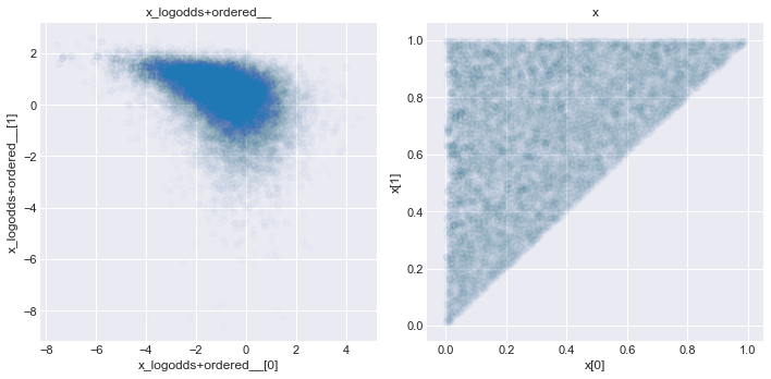
使用相同的方法, 我们也能从相同的分布当中创建有顺序的随机变量.比如, 我们能够使用 Chain 将 ordered 变换和 logodds 变换连接起来, 创建一个满足$x_{1}, x_{2} \sim Uniform (0,1)$ 且 $x_{1}<x_{2}$ 的 2D 随机变量.
Order = tr.Ordered()
Logodd = tr.LogOdds()
chain_tran = tr.Chain([Logodd, Order])

with pm.Model() as m0:
    x = pm.Uniform(
        'x', 0., 1., shape=2,
        transform=chain_tran,
        testval=[0.1, 0.9]
    )
    trace = pm.sample(5000, tune=1000, progressbar=False)

_, ax = plt.subplots(1, 2, figsize=(10, 5))
for ivar, varname in enumerate(trace.varnames):
    ax[ivar].scatter(trace[varname][:, 0], trace[varname][:, 1], alpha=.01)
    ax[ivar].set_xlabel(varname + '[0]')
    ax[ivar].set_ylabel(varname + '[1]')
    ax[ivar].set_title(varname)
plt.tight_layout()
Auto-assigning NUTS sampler...
Initializing NUTS using jitter+adapt_diag...
Multiprocess sampling (4 chains in 4 jobs)
NUTS: [x]
The acceptance probability does not match the target. It is 0.8793900638245146, but should be close to 0.8. Try to increase the number of tuning steps.
There was 1 divergence after tuning. Increase `target_accept` or reparameterize.
2.6 随机变量列表 / 多维随机变量
上面我们展示了如何创建不同尺度下的随机变量. 在很多模型当中, 你可能需要多个随机变量. 这里你可以使用 shape 参数:
with pm.Model() as model:
    x = pm.Normal('x', mu=0, sigma=1, shape=10)
如上所示, x 将会是一个长度为 10 的随机向量.
2.7 模型初始化的随机变量初始值
当 PyMC3 进行模型的初始化时, 会对随机变量生成一些初始值, 用于测试. 变量的测试值可以使用 test_value 属性来获取, 而对象中可以传入 testval 来进行测试变量的初始化:
with pm.Model():
    x = pm.Normal('x', mu=0, sigma=1, shape=5)

x.tag.test_value
array([0., 0., 0., 0., 0.])
with pm.Model():
    x = pm.Normal('x', mu=0, sigma=1, shape=5, testval=[0.1, 0.2, 0.3, 0.4, 0.5])

x.tag.test_value
array([0.1, 0.2, 0.3, 0.4, 0.5])
3. 接口
3.1 取样
PyMC3 中 MCMC 取样算法对函数是 pm.sample(). 如果不传入参数, 函数会默认选择最合适的采样器, 并自动初始化.
with pm.Model() as model:
    mu = pm.Normal('mu', mu=0, sigma=1)
    obs = pm.Normal('obs', mu=mu, sigma=1, observed=np.random.randn(100))

    trace = pm.sample(1000, tune=500)
Auto-assigning NUTS sampler...
Initializing NUTS using jitter+adapt_diag...
Multiprocess sampling (4 chains in 4 jobs)
NUTS: [mu]
Sampling 4 chains, 0 divergences: 100%|██████████| 6000/6000 [00:01<00:00, 5837.93draws/s]
The acceptance probability does not match the target. It is 0.8821243494848733, but should be close to 0.8. Try to increase the number of tuning steps.
正如你在上面看到的, PyMC3 自动选择了 NUTS 采样器, 这是一种对于复杂模型非常高效的采样工具. 同时, PyMC3 运行了不同的方法来寻找最佳的初始值. 这里我们从先验分布中采样了1000次, 并让采样器自行调整参数进行了500次迭代. 这500次采样默认情况下会被丢弃.
你也可以通过传入 cores 参数直接跑并行:
with pm.Model() as model:
    mu = pm.Normal('mu', mu=0, sigma=1)
    obs = pm.Normal('obs', mu=mu, sigma=1, observed=np.random.randn(100))

    trace = pm.sample(cores=12)
Auto-assigning NUTS sampler...
Initializing NUTS using jitter+adapt_diag...
Multiprocess sampling (12 chains in 12 jobs)
NUTS: [mu]
Sampling 12 chains, 0 divergences: 100%|██████████| 12000/12000 [00:02<00:00, 5107.82draws/s]
The acceptance probability does not match the target. It is 0.8823917312827685, but should be close to 0.8. Try to increase the number of tuning steps.
print(trace['mu'].shape)
print(trace.nchains)
print(trace.get_values('mu', chains=1).shape)
(6000,)
12
(500,)
你可以通过 pm.step_methods 来查看其他的采样器.
dir(pm.step_methods)
['BinaryGibbsMetropolis',
 'BinaryMetropolis',
 'CategoricalGibbsMetropolis',
 'CauchyProposal',
 'CompoundStep',
 'DEMetropolis',
 'ElemwiseCategorical',
 'EllipticalSlice',
 'HamiltonianMC',
 'LaplaceProposal',
 'Metropolis',
 'MultivariateNormalProposal',
 'NUTS',
 'NormalProposal',
 'PoissonProposal',
 'Slice',
 '__builtins__',
 '__cached__',
 '__doc__',
 '__file__',
 '__loader__',
 '__name__',
 '__package__',
 '__path__',
 '__spec__',
 'arraystep',
 'compound',
 'elliptical_slice',
 'gibbs',
 'hmc',
 'metropolis',
 'slicer',
 'step_sizes']
常用的步进采样法出了 NUTS 外, 还有 Metropolis 和 Slice . 对于大多数连续型随机变量的模型来说, NUTS 都是最好的方法. 对于一些非常复杂的模型, NUTS 采样会有些慢, 这时可以选择 Metropolis 方法来代替. 不过在实践中这种方法很难奏效. NUTS 在简单模型中采样非常快, 但是在复杂模型中和难以初始化的模型中会很慢. 对于某些复杂模型, NUTS 可能采样会比较慢. 虽然 Metropolis 会快一些, 然而采样效率会比较低, 抑或是难以得到理想的结果.
然而我们还是可以采用不同的采样方法, 甚至是不同的变量选择不同的采样方法.
with pm.Model() as model:
    mu = pm.Normal('mu', mu=0, sigma=1)
    sd = pm.HalfNormal('sd', sigma=1)
    obs = pm.Normal('obs', mu=mu, sigma=sd, observed=np.random.randn(100))

    step1 = pm.Metropolis(vars=[mu])
    step2 = pm.Slice(vars=[sd])
    trace = pm.sample(10000, step=[step1, step2], cores=12)
Multiprocess sampling (12 chains in 12 jobs)
CompoundStep
>Metropolis: [mu]
>Slice: [sd]
Sampling 12 chains, 0 divergences: 100%|██████████| 126000/126000 [00:21<00:00, 5961.49draws/s]
The number of effective samples is smaller than 25% for some parameters.
3.2 分析采样结果
我们最常用的方法是绘制 trace-plot
with model:
    pm.traceplot(trace);

我们也可以查看 Gelman-Rubin 统计量:
pm.gelman_rubin(trace)
Gelman-Rubin 统计量是一个现在广泛使用的 MCMC 模型诊断指标, 用以评估马尔可夫链是否收敛. 当链收敛时, 该值的目标分布应为 $N(0,1)$
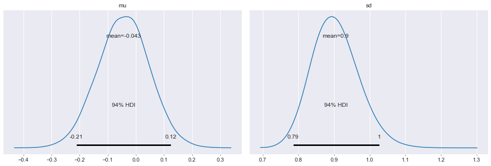
你还可以把后验分布画出来:
pm.plot_posterior(trace);
3.3 变分推断
PyMC3 支持变分推断技术. 该技术的估计过程会更快, 但是常常导致结果的精确性更低, 且结果有偏差. 该方法的实现主要是 pymc3.fit()
变分推断可以简单理解为如果没有办法得到目标的精确解, 我们通过不断迭代得到结果的近似解.
with pm.Model() as model:
    mu = pm.Normal('mu', mu=0, sigma=1)
    sd = pm.HalfNormal('sd', sigma=1)
    obs = pm.Normal('obs', mu=mu, sigma=sd, observed=np.random.randn(100))

    approx = pm.fit()
Average Loss = 148.81: 100%|██████████| 10000/10000 [00:02<00:00, 3385.39it/s]
Finished [100%]: Average Loss = 148.8
返回的估计结果和一般的采样结果一样, 仍然可以查看其后验分布等:
trace = approx.sample(500)
pm.traceplot(trace)
array([[<matplotlib.axes._subplots.AxesSubplot object at 0x7fa68aa81150>,
        <matplotlib.axes._subplots.AxesSubplot object at 0x7fa67a9c5ad0>],
       [<matplotlib.axes._subplots.AxesSubplot object at 0x7fa67a920590>,
        <matplotlib.axes._subplots.AxesSubplot object at 0x7fa658f70290>]],
      dtype=object)

4. 后验期望分布采样
sample_posterior_predictive() 函数通过对后验分布进行采样, 来提供对后验分布的检验.
对后验期望分布采样是验证模型非常好的一种方法, 其原理是对估计出的后验分布进行采样, 然后检验与观察数据之间的偏差. 期望进一步了解详情可以观看 https://www.youtube.com/watch?v=TMnXQ6G6E5Y 的视频)
data = np.random.randn(1000)

with pm.Model() as I_do_not_want_to_name_as_model:
    mu = pm.Normal('mu', 0, 1)
    sd = pm.HalfNormal('sd', 1)
    obs = pm.Normal('obs', mu=mu, sigma=sd, observed=data)

    trace = pm.sample()
Auto-assigning NUTS sampler...
Initializing NUTS using jitter+adapt_diag...
Multiprocess sampling (4 chains in 4 jobs)
NUTS: [sd, mu]
Sampling 4 chains, 0 divergences: 100%|██████████| 4000/4000 [00:00<00:00, 4593.40draws/s]
The acceptance probability does not match the target. It is 0.8829296376207753, but should be close to 0.8. Try to increase the number of tuning steps.
with I_do_not_want_to_name_as_model:
    post_pred = pm.sample_posterior_predictive(trace, samples=500)
100%|██████████| 500/500 [00:01<00:00, 362.26it/s]
post_pred['obs'].shape
(500, 1000)
fig, ax = plt.subplots()
sns.distplot(post_pred['obs'].mean(axis=1), label='Posterior predictive means', ax=ax)
ax.axvline(data.mean(), ls='--', color='r', label='True mean')
ax.legend();

Xiaokai Xia
Ph.D. candidate
A doctor of TCM with Data Science and Psychological Counseling is learning psychology.